“We’re Building Something, Here, Detective, We’re Building It From Scratch. All The Pieces Matter.” (Lester, The Wire)
Connection data
In this guide, we will use hemibrainr look at connectivity data for a starting neuron of interest. They neuron will be LHMB1 (Bates & Schlegel et al., 2020)), the only neuron from the ‘innate olfactory’ brain center of the fly (lateral horn), to innervate the ‘associative memory centre’ directly (mushroom body lobes). You can try re-running this analysis for any neuron of your interest.
We will use precomputed data from the hemibrainr Google team drive. In order to connect R to this Google drive, you have a few options. Please see this article. To see how to split neurons into axon and dendrite, without access to this drive, please see this article.
Load google drive
Let’s get hemibrainr and our Google drive loaded:
# Load package
library(hemibrainr)
library(ggplot2)

# Else, it wants to see it on the mounted team drive, here
options("remote_connectome_data")

# If this does not give a path to the hemibrainr google drive...
## But you do have access, and have set up rclone
### Try:
##### hemibrainr_rclone()
Find neuron of interest
First, let us find the beautiful LHMB1 neuron:
We now have our unique identifier, ‘body ID’, for LHMB1. We can use it to get hold of this neuron:
db = hemibrain_neurons() # This a neuronlistfh object read from the google drive
lhmb1.neuron = db[lhmb1.bodyid]

# Alternatively, without the drive:
## lhmb1.neuron = hemibrain_read_neurons(lhmb1.bodyid, remote = FALSE)
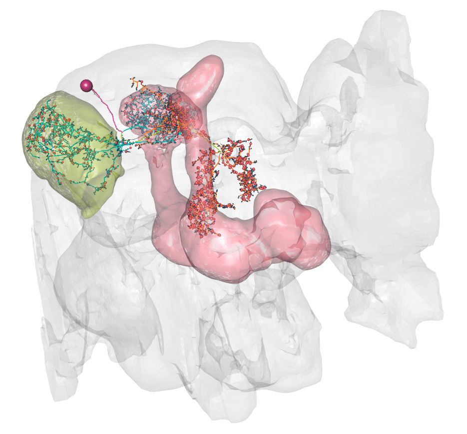
Let us confirm it is what we think it is, by plotting this neurons:
# Get ROIs
lhr = neuprint_ROI_mesh("LH(R)")
mbr = neuprint_ROI_mesh("MB(R)")

# Plot
nat::nopen3d()
hemibrain_view()
plot3d(lhr, alpha = 0.3, col = hemibrain_bright_colors["green"], add = TRUE)
plot3d(mbr, alpha = 0.3, col = hemibrain_bright_colors["pink"], add = TRUE)
plot3d(hemibrain.surf, alpha = 0.1, col = "lightgrey", add = TRUE)
plot3d_split(lhmb1.neuron, lwd =2, soma = 600)
So here you can see dendrite (blue) in the lateral horn (green volume) and calyx, and axon (orange) in the lobes of the mushroom body (pink volume).
Get neuron connectivity data
Now we can get a precomputed edgelist for the brain from the Google drive, which breaks down connections by axon and dendrite. By default this is read from an SQLite database on the Google drive. This means we can access the data, without loading a multi Gb .csv into memory:
# Get  the edgelist
elist = hemibrain_elist()

# Let's count a strong connection as one that is 10-synapses strong and/or account for at least 1% of the downstream arbour's postsynapses:
elist.strong = subset(elist, elist$count >= 10 | elist$norm >= 0.01)

# Get a lot of meta data for each hemibrain neuron
hemi.meta = hemibrain_meta()
In our elist, count is the number of synaptic connections between two arbours. The arbour types are given by Label and partner.Label. The neuron identities are given as pre, the upstream (source) neuron and post, the downstream (target) neuron. The value of norm is generated by taking count and dividing it by the total number of postsynapses on the downstream target’s given arbour (note, not all connection in the neuron!). See your article on neuron splitting, for more information.
We have the connectivity of the whole dataset at our fingertips. Or at least, all the large fragments that could be considered neurons (see ?hemibrain_bodyids). Let us have a quick look at what the distribution of different connection types is:
lhmb1.elist <- elist %>%
  dplyr::filter(pre == lhmb1.bodyid | post == lhmb1.bodyid, count > 10 | norm > 0.01) %>%
  mutate(feedback = ifelse( (post %in% .data$pre & post %in% .data$post)) & !post%in%lhmb1.bodyid ) %>%
  arrange(desc(norm), desc(count)) %>% # sort
  mutate(post.type = hemi.meta[match(post, hemi.meta$bodyid),"type"]) %>% # cell_type
  mutate(post.layer = hemi.meta[match(post, hemi.meta$bodyid),"ct.layer"]) %>% # 'layre' in the olfactory system
  mutate(pre.type = hemi.meta[match(pre, hemi.meta$bodyid),"type"]) %>%
  mutate(pre.layer = hemi.meta[match(pre, hemi.meta$bodyid),"ct.layer"]) %>%
  data.frame()
head(lhmb1.elist)